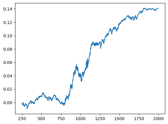
# Box 6.1 and Example 6.1: Finding Correlations between Returns of Different Time Framesimport numpy as npimport pandas as pd#import matplotlib.pyplot as plt#import statsmodels.formula.api as sm#import statsmodels.tsa.stattools as ts#import statsmodels.tsa.vector_ar.vecm as vmfrom scipy.stats import pearsonr# 用于计算最大回撤(Maximum Drawdown)和最大回撤持续时间(Maximum Drawdown Duration)def calculateMaxDD(cumret):# =============================================================================# calculation of maximum drawdown and maximum drawdown duration based on# cumulative COMPOUNDED returns. cumret must be a compounded cumulative return.# i is the index of the day with maxDD.# ============================================================================= highwatermark=np.zeros(cumret.shape) drawdown=np.zeros(cumret.shape) drawdownduration=np.zeros(cumret.shape)for t in np.arange(1, cumret.shape[0]): highwatermark[t]=np.maximum(highwatermark[t-1], cumret[t]) drawdown[t]=(1+cumret[t])/(1+highwatermark[t])-1if drawdown[t]==0: drawdownduration[t]=0else: drawdownduration[t]=drawdownduration[t-1]+1 maxDD, i=np.min(drawdown), np.argmin(drawdown) # drawdown < 0 always maxDDD=np.max(drawdownduration)return maxDD, maxDDD, idf=pd.read_csv('datas/inputDataOHLCDaily_TU_20120511.csv')df['Date']=pd.to_datetime(df['Date'], format='%Y%m%d').dt.date # remove HH:MM:SSdf.set_index('Date', inplace=True)# 计算不同时间框架下的收益率相关性:for lookback in [1, 5, 10, 25, 60, 120, 250]:for holddays in [1, 5, 10, 25, 60, 120, 250]: ret_lag=df.pct_change(periods=lookback) ret_fut=df.shift(-holddays).pct_change(periods=holddays,fill_method=None)if (lookback >= holddays): indepSet=range(0, ret_lag.shape[0], holddays)else: indepSet=range(0, ret_lag.shape[0], lookback) ret_lag=ret_lag.iloc[indepSet] ret_fut=ret_fut.iloc[indepSet]# 确保 ret_lag 和 ret_fut 是 pandas Series ret_lag = ret_lag.squeeze() # 将 DataFrame 转换为 Series ret_fut = ret_fut.squeeze() # 将 DataFrame 转换为 Series goodDates=(ret_lag.notna() & ret_fut.notna()).values (cc, pval)=pearsonr(ret_lag[goodDates], ret_fut[goodDates])print('%4i%4i%7.4f%7.4f'% (lookback, holddays, cc, pval))lookback=250holddays=25longs=df > df.shift(lookback)shorts=df < df.shift(lookback)pos=np.zeros(df.shape)pd.set_option('future.no_silent_downcasting', True)for h inrange(holddays-1): long_lag=longs.shift(h).fillna(False).astype(bool) short_lag=shorts.shift(h).fillna(False).astype(bool) pos[long_lag]=pos[long_lag]+1 pos[short_lag]=pos[short_lag]-1pos=pd.DataFrame(pos)pnl=np.sum((pos.shift().values)*(df.pct_change().values), axis=1) # daily P&L of the strategyret=pnl/np.sum(np.abs(pos.shift()), axis=1)cumret=(np.cumprod(1+ret)-1)cumret.plot()print('APR=%f Sharpe=%f'% (np.prod(1+ret)**(252/len(ret))-1, np.sqrt(252)*np.mean(ret)/np.std(ret)))maxDD, maxDDD, i=calculateMaxDD(cumret.fillna(0))print('Max DD=%f Max DDD in days=%i'% (maxDD, maxDDD))
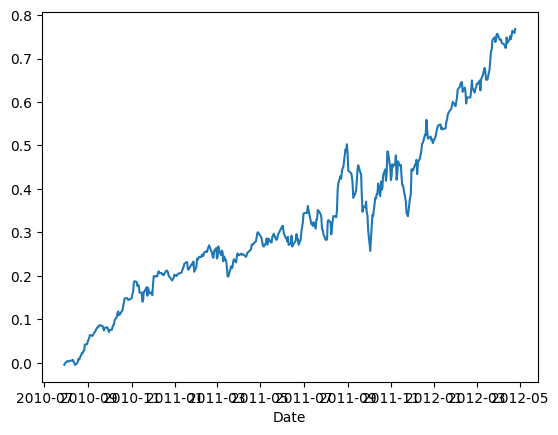
# Volatility Futures vs Equity Index Futuresimport numpy as npimport pandas as pd#import matplotlib.pyplot as plt#import statsmodels.formula.api as sm#import statsmodels.tsa.stattools as ts#import statsmodels.tsa.vector_ar.vecm as vmentryThreshold=0.1onewaytcost=1/10000# VX futuresvx=pd.read_csv('datas/inputDataDaily_VX_20120507.csv')vx['Date']=pd.to_datetime(vx['Date'], format='%Y%m%d').dt.date # remove HH:MM:SSvx.set_index('Date', inplace=True)# VIX indexvix=pd.read_csv('datas/VIX.csv')vix['Date']=pd.to_datetime(vix['Date'], format='%Y-%m-%d').dt.date # remove HH:MM:SSvix.set_index('Date', inplace=True)vix=vix[['Close']]vix.rename({'Close': 'VIX'}, axis=1, inplace=True)# ES backadjusted continuous contractes=pd.read_csv('datas/inputDataDaily_ES_20120507.csv')es['Date']=pd.to_datetime(es['Date'], format='%Y%m%d').dt.date # remove HH:MM:SSes.set_index('Date', inplace=True)es.rename({'Close': 'ES'}, axis=1, inplace=True)# Merge on common datesdf=pd.merge(vx, vix, how='inner', on='Date')df=pd.merge(df, es, how='inner', on='Date')vx=df.drop({'VIX', 'ES'}, axis=1)vix=df[['VIX']]es=df[['ES']]isExpireDate=vx.notnull() & vx.shift(-1).isnull()# Define front month as 40 days to 10 days before expirationnumDaysStart=40numDaysEnd=10positions=np.zeros((vx.shape[0], vx.shape[1]+1))for c inrange(vx.shape[1]-1): expireIdx=np.where(isExpireDate.iloc[:,c])if c==0: startIdx=expireIdx[0]-numDaysStart endIdx=expireIdx[0]-numDaysEndelse: startIdx=np.max((endIdx+1, expireIdx[0]-numDaysStart)) endIdx=expireIdx[0]-numDaysEndif (expireIdx[0] >=0):# startIdx = int(startIdx[0])# endIdx = int(endIdx[0])if(isinstance(startIdx, np.ndarray)): intStartIdx = startIdx[0]else: intStartIdx = startIdxif(isinstance(endIdx, np.ndarray)): intEndIdx = endIdx[0]else: intEndIdx = endIdx idx=np.arange(intStartIdx, intEndIdx+1)# print(expireIdx)# expireIdx = int(expireIdx[0])# print(expireIdx[0][0])# print(type(expireIdx))# temp = np.arange(expireIdx[0][0]-intStartIdx+1, expireIdx[0][0]-intEndIdx, -1) dailyRoll=(vx.iloc[idx, c]-vix.iloc[idx, 0])/np.arange(expireIdx[0][0]-intStartIdx+1, expireIdx[0][0]-intEndIdx, -1) positions[idx[dailyRoll > entryThreshold], c]=-1 positions[idx[dailyRoll > entryThreshold], -1]=-1 positions[idx[dailyRoll <-entryThreshold], c]=1 positions[idx[dailyRoll < entryThreshold], -1]=1y=pd.merge(vx*1000, es*50, on='Date')positions=pd.DataFrame(positions, index=y.index)pnl=np.sum((positions.shift().values)*(y-y.shift()) - onewaytcost*np.abs(positions.values*y - (positions.values*y).shift()), axis=1) # daily P&L of the strategyret=pnl/np.sum(np.abs((positions.values*y).shift()), axis=1)idx=ret.index[ret.index >= pd.to_datetime("2008-08-04").date()]cumret=(np.cumprod(1+ret[idx[500:]])-1)cumret.plot()print('APR=%f Sharpe=%f'% (np.prod(1+ret[idx[500:]])**(252/len(ret[idx[500:]]))-1, np.sqrt(252)*np.mean(ret[idx[500:]])/np.std(ret[idx[500:]])))# from calculateMaxDD import calculateMaxDDmaxDD, maxDDD, i=calculateMaxDD(cumret.fillna(0))print('Max DD=%f Max DDD in days=%i'% (maxDD, maxDDD))#APR=0.377914 Sharpe=2.117500#Max DD=-0.434420 Max DDD in days=73
APR=0.377914 Sharpe=2.117500
Max DD=-0.434420 Max DDD in days=73
C:\Users\win10\AppData\Local\Temp\ipykernel_4936\1180818726.py:22: FutureWarning: Series.__getitem__ treating keys as positions is deprecated. In a future version, integer keys will always be treated as labels (consistent with DataFrame behavior). To access a value by position, use `ser.iloc[pos]`
  highwatermark[t]=np.maximum(highwatermark[t-1], cumret[t])
C:\Users\win10\AppData\Local\Temp\ipykernel_4936\1180818726.py:23: FutureWarning: Series.__getitem__ treating keys as positions is deprecated. In a future version, integer keys will always be treated as labels (consistent with DataFrame behavior). To access a value by position, use `ser.iloc[pos]`
  drawdown[t]=(1+cumret[t])/(1+highwatermark[t])-1
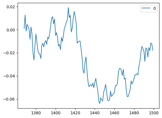
# Example 6.2: Cross-Sectional Momentum Strategy for Stocksimport numpy as npimport pandas as pd#import matplotlib.pyplot as plt#import statsmodels.formula.api as sm#import statsmodels.tsa.stattools as ts#import statsmodels.tsa.vector_ar.vecm as vmlookback=252holddays=25topN=50# Stockscl=pd.read_csv('datas/inputDataOHLCDaily_20120424_cl.csv')stocks=pd.read_csv('datas/inputDataOHLCDaily_20120424_stocks.csv')cl['Var1']=pd.to_datetime(cl['Var1'], format='%Y%m%d').dt.date # remove HH:MM:SScl.columns=np.insert(stocks.values, 0, 'Date')cl.set_index('Date', inplace=True)ret=cl.pct_change(periods=lookback)longs=np.full(cl.shape, False)shorts=np.full(cl.shape, False)positions=np.zeros(cl.shape)for t inrange(lookback, cl.shape[0]): hasData=np.where(np.isfinite(ret.iloc[t, :])) hasData=hasData[0]iflen(hasData)>0: idxSort=np.argsort(ret.iloc[t, hasData]) longs[t, hasData[idxSort.values[np.arange(-np.min((topN, len(idxSort))),0)]]]=1 shorts[t, hasData[idxSort.values[np.arange(0,topN)]]]=1longs=pd.DataFrame(longs)shorts=pd.DataFrame(shorts)for h inrange(holddays-1): long_lag=longs.shift(h).fillna(False).astype(bool) short_lag=shorts.shift(h).fillna(False).astype(bool) positions[long_lag]=positions[long_lag]+1 positions[short_lag]=positions[short_lag]-1positions=pd.DataFrame(positions)ret=pd.DataFrame(np.sum((positions.shift().values)*(cl.pct_change().values), axis=1)/(2*topN)/holddays) # daily P&L of the strategycumret=(np.cumprod(1+ret)-1)cumret.plot()print('APR=%f Sharpe=%f'% (np.prod(1+ret)**(252/len(ret))-1, np.sqrt(252)*np.mean(ret,axis=0)/np.std(ret)))#from calculateMaxDD import calculateMaxDD#maxDD, maxDDD, i=calculateMaxDD(cumret.fillna(0))#print('Max DD=%f Max DDD in days=%i' % (maxDD, maxDDD))
APR=-0.003019 Sharpe=-0.286628
C:\Users\win10\AppData\Roaming\Python\Python39\site-packages\numpy\_core\fromnumeric.py:84: FutureWarning: The behavior of DataFrame.prod with axis=None is deprecated, in a future version this will reduce over both axes and return a scalar. To retain the old behavior, pass axis=0 (or do not pass axis)
  return reduction(axis=axis, out=out, **passkwargs)
C:\Users\win10\AppData\Roaming\Python\Python39\site-packages\numpy\_core\fromnumeric.py:3800: FutureWarning: The behavior of DataFrame.std with axis=None is deprecated, in a future version this will reduce over both axes and return a scalar. To retain the old behavior, pass axis=0 (or do not pass axis)
  return std(axis=axis, dtype=dtype, out=out, ddof=ddof, **kwargs)
C:\Users\win10\AppData\Local\Temp\ipykernel_4936\4244792157.py:49: FutureWarning: Calling float on a single element Series is deprecated and will raise a TypeError in the future. Use float(ser.iloc[0]) instead
  print('APR=%f Sharpe=%f' % (np.prod(1+ret)**(252/len(ret))-1, np.sqrt(252)*np.mean(ret,axis=0)/np.std(ret)))
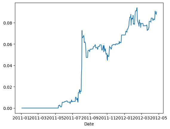
# Example 7.1: Opening Gap Strategy for FSTXimport numpy as npimport pandas as pd#import matplotlib.pyplot as pltentryZscore=0.1df=pd.read_csv('datas/inputDataDaily_FSTX_20120517.csv')df['Date']=pd.to_datetime(df['Date'], format='%Y%m%d').dt.date # remove HH:MM:SSdf.set_index('Date', inplace=True)stdretC2C90d=df['Close'].pct_change().rolling(90).std().shift()longs= df['Open'] >= df['High'].shift()*(1+entryZscore*stdretC2C90d)shorts=df['Open'] >= df['Low'].shift()*(1-entryZscore*stdretC2C90d)positions=np.zeros(longs.shape)positions[longs]=1positions[shorts]=-1ret=positions*(df['Close']-df['Open'])/df['Open']cumret=(np.cumprod(1+ret)-1)cumret.plot()print('APR=%f Sharpe=%f'% (np.prod(1+ret)**(252/len(ret))-1, np.sqrt(252)*np.mean(ret)/np.std(ret)))# from calculateMaxDD import calculateMaxDDmaxDD, maxDDD, i=calculateMaxDD(cumret.fillna(0))print('Max DD=%f Max DDD in days=%i'% (maxDD, maxDDD))#APR=0.074864 Sharpe=0.494857#Max DD=-0.233629 Max DDD in days=789
APR=0.074864 Sharpe=0.494857
Max DD=-0.233629 Max DDD in days=789
C:\Users\win10\AppData\Local\Temp\ipykernel_4936\1180818726.py:22: FutureWarning: Series.__getitem__ treating keys as positions is deprecated. In a future version, integer keys will always be treated as labels (consistent with DataFrame behavior). To access a value by position, use `ser.iloc[pos]`
  highwatermark[t]=np.maximum(highwatermark[t-1], cumret[t])
C:\Users\win10\AppData\Local\Temp\ipykernel_4936\1180818726.py:23: FutureWarning: Series.__getitem__ treating keys as positions is deprecated. In a future version, integer keys will always be treated as labels (consistent with DataFrame behavior). To access a value by position, use `ser.iloc[pos]`
  drawdown[t]=(1+cumret[t])/(1+highwatermark[t])-1
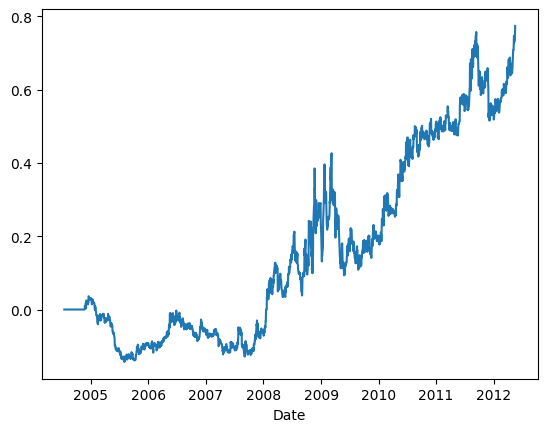
# Example 4.1: Buy-on-Gap Model on SPX Stocksimport numpy as npimport pandas as pd#import matplotlib.pyplot as plt#import statsmodels.formula.api as sm#import statsmodels.tsa.stattools as ts#import statsmodels.tsa.vector_ar.vecm as vmop=pd.read_csv('datas/inputDataOHLCDaily_20120424_op.csv')cl=pd.read_csv('datas/inputDataOHLCDaily_20120424_cl.csv')stocks=pd.read_csv('datas/inputDataOHLCDaily_20120424_stocks.csv')op['Var1']=pd.to_datetime(op['Var1'], format='%Y%m%d').dt.date # remove HH:MM:SSop.columns=np.insert(stocks.values, 0, 'Date')op.set_index('Date', inplace=True)cl['Var1']=pd.to_datetime(cl['Var1'], format='%Y%m%d').dt.date # remove HH:MM:SScl.columns=np.insert(stocks.values, 0, 'Date')cl.set_index('Date', inplace=True)earnann=pd.read_csv('datas/earnannFile.csv')earnann['Date']=pd.to_datetime(earnann['Date'], format='%Y%m%d').dt.date # remove HH:MM:SSearnann.set_index('Date', inplace=True)np.testing.assert_array_equal(stocks.iloc[0,:], earnann.columns)df=pd.merge(op, cl, how='inner', left_index=True, right_index=True, suffixes=('_op', '_cl'))df=pd.merge(earnann, df, how='inner', left_index=True, right_index=True)earnann=df.iloc[:, 0:(earnann.shape[1])].astype(bool)op=df.iloc[:, (earnann.shape[1]):((earnann.shape[1])+op.shape[1])]cl=df.iloc[:, ((earnann.shape[1])+op.shape[1]):]op.columns=stocks.iloc[0,:]cl.columns=stocks.iloc[0,:]lookback=90retC2O=(op-cl.shift())/cl.shift()stdC2O=retC2O.rolling(lookback).std()positions=np.zeros(cl.shape) longs= (retC2O >=0.5*stdC2O) & earnannshorts= (retC2O <=-0.5*stdC2O) & earnannpositions[longs]=1positions[shorts]=-1ret=np.sum(positions*(cl-op)/op, axis=1)/30cumret=(np.cumprod(1+ret)-1)cumret.plot()print('APR=%f Sharpe=%f'% (np.prod(1+ret)**(252/len(ret))-1, np.sqrt(252)*np.mean(ret)/np.std(ret)))# from calculateMaxDD import calculateMaxDDmaxDD, maxDDD, i=calculateMaxDD(cumret.fillna(0))print('Max DD=%f Max DDD in days=%i'% (maxDD, maxDDD))#APR=0.068126 Sharpe=1.494743#Max DD=-0.026052 Max DDD in days=109
APR=0.068126 Sharpe=1.494743
Max DD=-0.026052 Max DDD in days=109
C:\Users\win10\AppData\Local\Temp\ipykernel_4936\1180818726.py:22: FutureWarning: Series.__getitem__ treating keys as positions is deprecated. In a future version, integer keys will always be treated as labels (consistent with DataFrame behavior). To access a value by position, use `ser.iloc[pos]`
  highwatermark[t]=np.maximum(highwatermark[t-1], cumret[t])
C:\Users\win10\AppData\Local\Temp\ipykernel_4936\1180818726.py:23: FutureWarning: Series.__getitem__ treating keys as positions is deprecated. In a future version, integer keys will always be treated as labels (consistent with DataFrame behavior). To access a value by position, use `ser.iloc[pos]`
  drawdown[t]=(1+cumret[t])/(1+highwatermark[t])-1
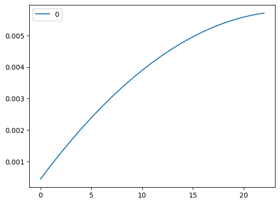
# Box 8.1import numpy as npimport pandas as pd#from scipy.stats import describe from scipy.stats import pearson3#import matplotlib.pyplot as plt#import statsmodels.formula.api as sm#import statsmodels.tsa.stattools as ts#import statsmodels.tsa.vector_ar.vecm as vmfrom scipy.optimize import minimizedf=pd.read_csv('datas/AUDCAD_unequal_ret.csv')# 使用pearson3函数拟合数据,并计算了数据的偏度、位置和尺度参数skew_, loc_, scale_=pearson3.fit(df) print('skew=%f loc=%f scale=%f'% (skew_, loc_, scale_))mean,var,skew,kurt=pearson3.stats(skew_, loc_, scale_, moments='mvks')print('mean=%f var=%f skew=%f kurt=%f'% (mean, var, skew, kurt))# 使用拟合得到的参数生成了100,000个模拟收益率ret_sim=pearson3.rvs(skew_, loc_, scale_, size=100000, random_state=0)# 定义了一个函数g,用于计算给定收益率和杠杆率的增长率def g(f, R):return np.sum(np.log(1+f*R), axis=0)/R.shape[0]# 对于不同的杠杆率(从1到23),计算了模拟收益率的增长率,并绘制了图表myf=range(1, 24)myg=np.full(24, np.nan)for f in myf: myg[f]=g(f, ret_sim)myg=myg[1:]myg=pd.DataFrame(myg)myg.plot()# 定义了一个最小化函数minusG和minusGsim,用于找到最优的杠杆率minusG =lambda f : -g(f, df)minusGsim =lambda f : -g(f, ret_sim)# 使用minimize函数找到了最优的杠杆率和对应的最大增长率#optimal leverage based on simulated returnsres = minimize(minusGsim, 0, method='Nelder-Mead')optimalF=res.xprint('Optimal leverage=%f optimal growth rate=%f'% (optimalF[0], -res.fun))#Optimal leverage=25.512625 optimal growth rate=0.005767minR=np.min(ret_sim)print('minR=%f'% (minR))#minR=-0.018201# max drawdown with optimal leverage# from calculateMaxDD import calculateMaxDDmaxDD, maxDDD, i=calculateMaxDD((np.cumprod(1+optimalF*ret_sim)-1))print('Max DD=%f with optimal leverage=%f'% (maxDD, optimalF[0]))#Max DD=-0.996312 with optimal leverage=25.512625#max drawdown with half of optimal leveragemaxDD, maxDDD, i=calculateMaxDD((np.cumprod(1+optimalF/2*ret_sim)-1))print('Max DD=%f with half optimal leverage=%f'% (maxDD, optimalF[0]/2))#Max DD=-0.900276 with half optimal leverage=12.756313# max drawdown with 1/7 of optimal leveragemaxDD, maxDDD, i=calculateMaxDD((np.cumprod(1+optimalF/7*ret_sim)-1))print('Max DD=%f with half optimal leverage=%f'% (maxDD, optimalF[0]/7))#Max DD=-0.429629 with half optimal leverage=3.644661#max drawdown with 1/1.4 of optimal leverage for historical returnsmaxDD, maxDDD, i=calculateMaxDD((np.cumprod(1+optimalF/1.4*df.values)-1))print('Max DD=%f with historical returns=%f'% (maxDD, optimalF[0]/1.4))#Max DD=-0.625894 with historical returns=18.223304D=0.5print('Growth rate on simulated returns using D=%3.1f of optimal leverage on full account=%f'% (D, -minusGsim(optimalF*D)))#Growth rate on simulated returns using D=0.5 of optimal leverage on full account=0.004317maxDD, maxDDD, i=calculateMaxDD((np.cumprod(1+optimalF*D*ret_sim)-1))print('MaxDD on simulated returns using D of optimal leverage on full account=%f'% (maxDD))#MaxDD on simulated returns using D of optimal leverage on full account=-0.900276# 使用CPPI策略计算了模拟收益率和历史收益率的增长率和最大回撤# CPPIg_cppi=0drawdown=0for t inrange(ret_sim.shape[0]): g_cppi+=np.log(1+ret_sim[t]*D*optimalF*(1+drawdown)) drawdown=min([0, (1+drawdown)*(1+ret_sim[t])-1])g_cppi=g_cppi/len(ret_sim)print('Growth rate on simulated returns using CPPI=%f'% g_cppi[0])#Growth rate on simulated returns using CPPI=0.004264print('Growth rate on historical returns using D of optimal leverage on full account=%f'% (-minusG(optimalF*D)))#Growth rate on historical returns using D of optimal leverage on full account=0.004053maxDD, maxDDD, i=calculateMaxDD((np.cumprod(1+optimalF*D*df.values)-1))print('MaxDD on historical returns using D of optimal leverage on full account=%f'% (maxDD))#MaxDD on historical returns using D of optimal leverage on full account=-0.303448# CPPIg_cppi=0drawdown=0for t inrange(df.shape[0]): g_cppi+=np.log(1+df.iloc[t,]*D*optimalF*(1+drawdown))# print("=========")# print(type((1+drawdown)*(1+df.iloc[t,])-1))# print((1+drawdown)*(1+df.iloc[t,])-1)# print(((1+drawdown)*(1+df.iloc[t,])-1)[0])# print("=========") drawdown=np.min([0, ((1+drawdown)*(1+df.iloc[t,])-1)[0]])g_cppi=g_cppi/len(df)print('Growth rate on historical returns CPPI=%f'% (g_cppi))
skew=0.122820 loc=0.000432 scale=0.004231
mean=0.000432 var=0.000018 skew=0.122820 kurt=0.022627
Optimal leverage=25.512625 optimal growth rate=0.005767
minR=-0.018201
Max DD=-0.996312 with optimal leverage=25.512625
Max DD=-0.900276 with half optimal leverage=12.756313
Max DD=-0.429629 with half optimal leverage=3.644661
Max DD=-0.625894 with historical returns=18.223304
Growth rate on simulated returns using D=0.5 of optimal leverage on full account=0.004317
MaxDD on simulated returns using D of optimal leverage on full account=-0.900276
Growth rate on simulated returns using CPPI=0.004264
Growth rate on historical returns using D of optimal leverage on full account=0.004053
MaxDD on historical returns using D of optimal leverage on full account=-0.482626
C:\Users\win10\AppData\Local\Temp\ipykernel_4936\158564989.py:85: FutureWarning: Calling float on a single element Series is deprecated and will raise a TypeError in the future. Use float(ser.iloc[0]) instead
  print('Growth rate on historical returns using D of optimal leverage on full account=%f' % (-minusG(optimalF*D)))
C:\Users\win10\AppData\Local\Temp\ipykernel_4936\158564989.py:101: FutureWarning: Series.__getitem__ treating keys as positions is deprecated. In a future version, integer keys will always be treated as labels (consistent with DataFrame behavior). To access a value by position, use `ser.iloc[pos]`
  drawdown=np.min([0, ((1+drawdown)*(1+df.iloc[t,])-1)[0]])
Growth rate on historical returns CPPI=0.003991
C:\Users\win10\AppData\Local\Temp\ipykernel_4936\158564989.py:104: FutureWarning: Calling float on a single element Series is deprecated and will raise a TypeError in the future. Use float(ser.iloc[0]) instead
  print('Growth rate on historical returns CPPI=%f' % (g_cppi))